

The first two articles in this three-part series provided background and introduced you to the Retirement Income Modeling Tool (RIMT). The articles and instructions on the Tool website cover almost everything you need to know, and you can contact me directly with specific questions (or issues—remember, it’s still in “beta mode”).
To help you get more familiar with the tool, its capabilities, and how you might use it for your own situation, including inputting your specific information and interpreting the results, I’ll walk you through a case study in this article. I’ll also create variations for the case based on different assumptions to help illustrate the Tool’s capabilities. And each time, I’ll run the numbers (using the two different modeling methods), show you the results, and explain what they mean in real life.
First, another word of caution. This tool isn’t a precise forecast of what will happen; it simulates what could happen based on the inputs and assumptions you use, and those assumptions can have a major impact one way or the other. It’s intended to be informational and may be illuminating, but it should not be taken as fact or as financial or tax advice. Since it’s still a “work in progress” and I am continually improving it, I can’t claim 100% accuracy. Other tools have been professionally designed, developed, and rigorously tested, and they may be better for your situation. This one is mainly for those already in retirement who are wondering about longevity risk and want to better understand the dynamics of the bucket strategy (and the total return strategy as an alternative) and how they might play out with RMDs, QCDs, taxes, Social Security survivor benefits, and the possible use of QLACs for longevity protection. I have written about all of these in the past, and this tool brings them all together in a cohesive mathematical model.
Case study: optimistic scenario
This example is a 70-year-old couple who have saved for retirement and live modestly, perhaps (probably) like many of you. Because they saved diligently and were in a higher tax bracket while working, they ended up with a sizeable, but not huge, Traditional IRA balance. They are also both receiving Social Security benefits (Spouse 1—primary benefit, Spouse 2—spousal benefit). (If Spouse 2 is also receiving their PIA benefit, the Tool takes that into account when making the survivor calculation.) This will be our baseline scenario for modeling their cash flow into their 80s and 90s using the RIMT.
We’ll also look at variations of this scenario when “life happens”: the impact that higher inflation, some “market shocks,” and more conservative return estimates have on their situation. But we’ll start with an optimistic one—stable inflation and taxes, and moderate, consistent market returns. We’ll assume the couple uses the “bucket strategy” to manage withdrawals, as I explained in a previous article and in the Tool’s instruction manual. (The Tool also gives you the option to use a “total return strategy” instead—that’s activated by using the toggle button in Section 2. Both are totally acceptable retirement income strategies, although some tend to favor one over the other. Personally, I like the bucket strategy, but others lean the other way.)
Input page
Sections 1 through 3:

Sections 4 through 6:
In this case, as shown in Section 4, Spouse 1’s lifespan is estimated to be 10 years less (to age 85) than Spouse 2’s (to age 95). We all know it’s not uncommon for one spouse to predecease the other, and I chose those ages for illustrative purposes. Current actuarial tables suggest that a healthy 70-year-old couple could live well into their 80s, and there is a 1-in-2 statistical probability that at least one of them will live into their 90s. However, we must always remind ourselves that our lives are in God’s hands, and he has set the time of our transition into eternity.
Remember, Section 6 (Return Assumptions)—your expected “fixed rate” return—is the average annual return applied to each asset “bucket” in the portfolio, each year, over the life of the portfolio. In this case, we’re using ‘moderate’ return assumptions; there are also ‘conservative’ and ‘custom’ (you set the values) return presets. You can override this by using the Monte Carlo simulation option (toggle ‘on’ in Section 15).

Sections 7 through 15

Results
Normal “fixed rate of return assumptions” simulation:

“Fixed Rate Assumptions” graphics:

“Fixed Rate Assumptions” tables (2 of the 4 tables that you can display):


Monte Carlo simulation:
Unlike the “fixed rate return” assumptions, this simulation uses variable annual return assumptions based on historical data and a probability distribution. This overrides any market “shocks” that you may have introduced, but that was not the case in this scenario. You can run up to 3,000 trials in the simulation.

Monte Carlo simulation results:


Observations
Needless to say, this couple, with one spouse living to the ripe old age of 95, is in pretty good shape based on a fairly optimistic set of assumptions. Their portfolio holds up very well, and only the fixed-rate assumptions show the surviving spouse having to start withdrawing from equities at age 94. Based on the balance at that time, they’d still be fine if one or both of them made it to 100. Their portfolio is never fully depleted; in fact, with “moderate” returns, no major market shocks, and stable, relatively low tax rates, they could reach age 95 with about $500,000 based on both simulations. But you don’t need me to tell you this is an overly optimistic scenario. So let’s look at a less optimistic scenario for the same couple, what we’ll call the “life happens” scenario.
By the way, this scenario didn’t use the QCD option for charitable giving, so here’s what the simulations would have shown if it had. In the early years of this scenario, the RMD is actually smaller than what’s needed for spending, and once Social Security is added, the two combine to just a little more than what’s needed. That small surplus amount is the most efficient use of a QCD—giving away up to that amount doesn’t shrink the portfolio at all, since the money had to be withdrawn from the IRA anyway, but it does mean less spendable cash lands in the couple’s pocket than if they’d simply saved it, perhaps in a taxable brokerage or savings account. The upside is that the money is untaxed entirely rather than having to pay tax on it first and then giving away what’s left over. Giving more than that surplus amount starts drawing down the portfolio for real, since it’s money that would otherwise have stayed invested. But either way, a QCD tends to be the smarter way to give than withdrawing the money and writing a check yourself, since a QCD avoids the tax bill automatically, while a cash donation only helps at tax time if a couple itemizes deductions, and many don’t.
A “life happens” scenario
We all know that “life happens” because many of the things we held constant in the optimistic scenario will likely change, and not always for the best. So, for this scenario, the first big change is that the surviving spouse lives to age 100. A long shot, perhaps (statistically, there’s roughly a 20% to 30% chance that someone who lives into their 90s will make it to 100), but it can happen. We’ll assume that inflation runs higher at 3%, and instead of “moderate” market returns, we plan for “conservative” returns (still positive, but a little lower). We’ll also assume that tax rates don’t stay stable—at taxable income of $40,000, rates increase in both the lower and higher brackets. Finally, we introduce a couple of market shocks into the equation, similar to 2008 and 2022-2023.
Input page
Sections 1 through 3, 11, 12, & 14:


Results
Fixed Rate Assumption:


Monte Carlo simulation:


Observations
As you can see, what happened is what we might have expected: both runs show the surviving spouse having trouble somewhere between ages 97 and 100. In the Monte Carlo simulation, the portfolio survival rate probability to age 100 is fairly low (~32%). I wouldn’t call this an absolute “worst-case” scenario, but it’s much less favorable than the optimistic one, and it clearly illustrates how changing your assumptions can produce a very different result.
Higher inflation, lower Social Security benefits, and “market shocks” that depleted the investment portfolio forced the surviving spouse to start tapping equity based on the two simulations at age 93 and 89, respectively, and it was exhausted by age 98 and 100. When the portfolio is at zero, nothing remains in any asset bucket—cash, bonds, equity, Roth—to draw from. In reality, this household’s spendable income in those years is just Social Security of $72,818 by age 100, a substantial shortfall against the target income. The year-by-year details table above reflects this by “going into the red” at age 100. The “net withdrawal” (and therefore income) drops significantly from prior years because the equity assets have been exhausted.s
Input—QLAC
One way to mitigate portfolio depletion in this kind of scenario is to purchase a qualified longevity annuity contract (QLAC). In this scenario, we’ll assume the couple purchases a $200,000 QLAC from the core bonds bucket at age 70, with payouts beginning at age 85 and continuing for life. (I used a very conservative 25% annual payout number—25% with no COLA. However, the range based on current interest rates could be 25 to 30%. A higher payout would increase the median ending portfolio balance.)
Section 7:

Results
Monte Carlo simulation:


Observations
This brings us full circle to my first article about this tool and Mike Piper’s article on QLACs. He said QLACs can help in some situations, and this is one of them, as longevity protection improves significantly (to 60% at age 100). With the addition of the QLAC, the portfolio survives in most trials, and even if it didn’t, Social Security and annuity income would still total $122,818 at age 100, significantly higher than just Social Security alone.
I would be remiss not to mention home equity, which may be the “asset of last resort” for some retirees. I didn’t include it in the model as it is a highly illiquid asset that can only be “tapped” by selling or mortgaging (including refinancing, second mortgages, and reverse mortgages). If you have a lot of home equity (many retirees do), it may be just the thing to fill the gap if other assets run out too soon, especially if significant health care or long-term care expenses come into play. Keep that in mind, especially if you run your numbers and things start looking shaky in your 80s or early 90s.
Being able to model this kind of less-than-optimistic scenario is one reason I created this tool. As you can see, a lot changes when Spouse 1 passes away at age 85, regardless of what happens to the market, taxes, and inflation. And if Spouse 2 lives well into their 90s, or even to 100, that can put a lot of stress on a portfolio. A deferred annuity is a good way to relieve some of that stress, and the tool modeled it well.
Update 09/11/26 (improvements to tool)
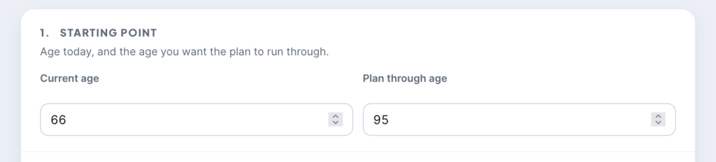
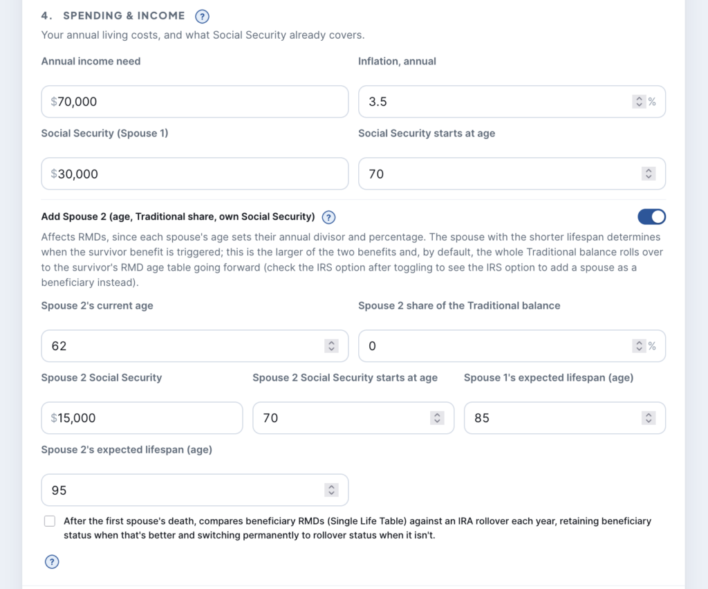
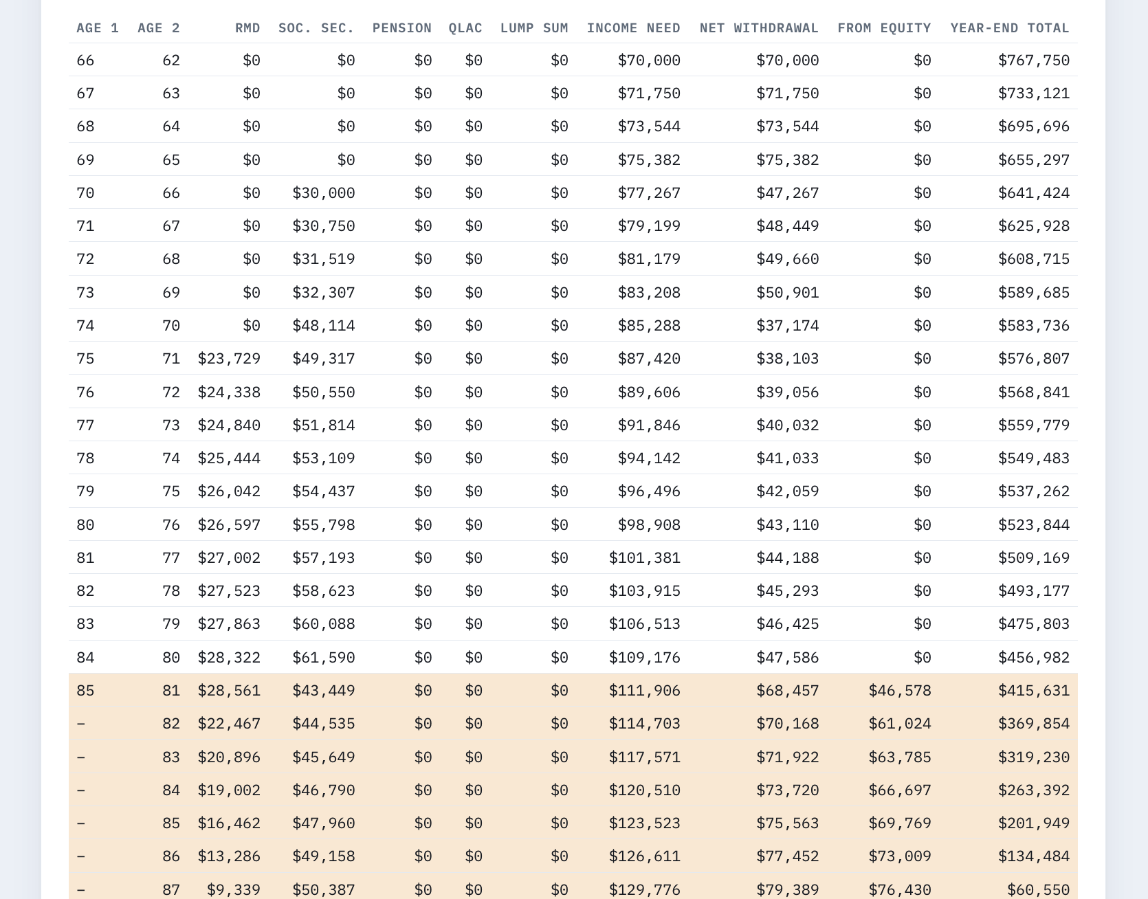
Shortly after publishing this article, a reader pointed out a limitation that I have since addressed and added to the tool: the ability to model different Social Security benefit start ages. Now the tool lets you specify the age and, when there’s a difference, model it in the simulation. The tables now display “Age 1” (for Spouse 1) and “Age 2” (for Spouse 2). I also added them to the “Quick Check” inputs screen. Here’s the new input screen and results tables that reflect these changes (note that setting Spouse 1’s age at 66 means RMDs start at age 75, not 73):
Try the tool here: Retirement Income Modeling Tool